- Research
- Open access
- Published:
Revealing influence of model structure and test case profile on the prioritization of test cases in the context of model-based testing
Journal of Software Engineering Research and Development volume 3, Article number: 1 (2015)
Abstract
Background
Test case prioritization techniques aim at defining an order of test cases that favor the achievement of a goal during test execution, such as revealing failures as earlier as possible. A number of techniques have already been proposed and investigated in the literature and experimental results have discussed whether a technique is more successful than others. However, in the context of model-based testing, only a few attempts have been made towards either proposing or experimenting test case prioritization techniques. Moreover, a number of factors that may influence on the results obtained still need to be investigated before more general conclusions can be reached.
Methods
In order to evaluate factors that potentially affect the performance of test case prioritization techniques, we perform three empirical studies, an exploratory one and two experiments. The first study focus on expose the techniques to a common and fair environment, since the investigated techniques have never been studied together, and observe their behavior. The following two experiments aim at observing the effects of two factors: the structure of the model and the profile of the test cases that fail. We designed the experiments using the one-factor-at-a-time strategy.
Results
The first study suggests that the investigated techniques performs differently, however other factors, aside from the test suites and number of failures, affect the techniques, motivating further investigation. As results from the two experiments, on one hand, the model structure do not affect significantly the investigated techniques. On the other hand, we are able to state that the profile of the test case that fails may have a definite influence on the performance of the techniques investigated.
Conclusions
Through these studies, we conclude that, a fair evaluation involving test case prioritization techniques must take into account, in addition to the techniques and the test suites, different characteristics of the test cases that fail as variable.
1 Introduction
The artifacts produced and the modifications applied during software development and evolution are usually validated by executing test cases. Often, the produced test suites are also subject to extensions and modifications, making management a difficult task. Moreover, their use may become increasingly less effective due to the difficulty to abstract and obtain information from test execution. For instance, if test cases that fail are either run too late or are difficult to locate due to the size and complexity of the suite.
To cope with this problem, a number of techniques have been proposed in the literature; they may be classified as test case selection, test suite reduction and test case prioritization. The general test case selection problem is concerned with selecting a subset of the test cases according to a specific (stop) criterion, whereas test suite reduction techniques focus on selecting a subset of the test cases, but the selected subset must provide the same requirement coverage as the original suite (Harrold et al. 1993). While the goal of selection and reduction is to produce a more cost-effective test suite, studies presented in the literature show that the techniques may not work effectively, since they discard test cases and consequently, some failures may not be revealed (Jeffrey and Gupta 2007).
On the other hand, test case prioritization techniques have been investigated in order to address the problem of defining an execution order of the test cases according with a given testing goal, particularly, detecting failures as early as possible (Rothermel et al. 1999). These techniques are suitable for general development context or in a more specific context, such as regression testing, depending on the information considered by the techniques (Rothermel et al. 2001). Moreover, both code-based and specification-based test suites may be handled, although, most techniques presented in the literature have been defined and evaluated for code-based suites in the context of regression testing (Elbaum et al. 2002) (Jiang et al. 2009).
Model-based Testing (MBT) is an approach to automate the design and generation of black-box test cases from specification models with all oracle information needed (Utting and Legeard 2007). MBT may operate with any model with different purposes and at different testing levels. As usually, automatic generation produces a huge amount of test cases that may also have a considerable degree of redundancy (Cartaxo et al. 2008, 2011).
Techniques for ordering the test cases may be required to support test case selection, for instance, to address constrained costs of running and analyzing the complete test suite and to improve the rate of failure detection. However, to the best of our knowledge, there are only few attempts presented in the literature to define test case prioritization techniques based on model information (Korel et al. 2008) (Gopinathan and Mohanty 2009). Generally, empirical studies are preliminary, making it difficult to assess current limitations and applicability of the techniques in the MBT context.
To provide useful information for the development of prioritization techniques, empirical studies must focus on controlling and/or observing factors that may determine the success of a given technique. Considering the goals of prioritization in the context of MBT, a number of factors can be determinant such as the size and the coverage of the suite, the structure of the model (that may determine the size and structure of test cases), the amount and distribution of failures and the degree of redundancy of test cases.
In this paper, we investigate the influence of two factors: the structure of the model and the profile of the test cases that fail. For this, we conduct three empirical studies, where real application models, as well as automatically generated ones, are considered. The focus is on general prioritization techniques suitable to MBT test suites. We represent the system level behavior through Labeled Transition Systems - LTS.
The purpose of the first study is to acquire preliminary observations by considering real application models. From this study, we conclude that a number of different factors might influence on the performance of the techniques. Therefore, the purpose of the second and third studies, the main contribution of this paper, is to investigate specific factors by controlling them through synthetic models.
In the studies, we considered four prioritization techniques: Adaptive Random Testing (ART) (Chen et al. 2004) with two different distance functions, producing two variant techniques named ART_Jac (Jaccard distance) and ART_Man (Manhattan distance); Fixed Weights (Gopinathan and Mohanty 2009) and STOOP (Gopinathan and Mohanty 2009).
This paper is an extension of the work presented by Ouriques et al. (2013). We extend it by: i) providing an example to illustrate the impacts of external factors over the techniques; ii) considering two more techniques in the second and third performed experiments (in the original paper, only ART_Jac and STOOP are considered); and iii) replicating the second and the third experiments, using new samples, better explained in the correspondent sections.
The conclusions of the replication of the experiments discussed in this paper, point to the same direction of the results already presented in the previous work. Despite the fact that the structure of the models may present or not certain constructions (for instance the presence of loopsa), it is not possible to differentiate the performance of the techniques when focusing on the presence of the construction investigated. On the other hand, depending on the profile of the test cases that fail (longest, shortest, essential, and so on), one technique may perform better than the other one, leading to some influence of this factor.
The studies presented in this paper focus on system level models, represented as activity diagrams and/or LTS with inputs and outputs as transitions. We generate synthetic models according to the strategy presented by Oliveira Neto et al. (2013). Test cases are sequences of transitions extracted from a model by a depth-search algorithm as presented by Cartaxo et al. (2011) and Sapna and Mohanty (2009). Prioritization techniques receive as input a test suite and produce as output an ordering for the test cases.
The paper presents the following structure. Section 1 exposes fundamental concepts, along with a quick definition of the prioritization techniques considered in this paper and discusses the related works. Section 1 presents a motivating example, showing the performance of three test case prioritization strategies. Section 1 shows a preliminary study where techniques are investigated in the context of two real applications, varying the amount of failures. Sections 1 and 1 present the main empirical studies conducted: the former reports a study with automatically generated models, in which we control the presence of certain structural constructions, whereas the latter depicts a study that we investigated different profiles of the test case that fails, also using synthetic models. Section 1 presents concluding remarks about the results obtained and pointers for further research. Details about the input models and data collected in the studies are available at the project site (Ouriques et al. 2015). We defined and planned the empirical studies according to the general framework proposed by Wohlin et al. (2000) and used the R tool (Gentleman and Ihaka 2015) to support data analysis.
2 Background
This section presents the test case prioritization concept (Subsection 1), details about the techniques considered in this paper (Subsection 1) and the related work (Subsection 1).
2.1 Test case prioritization
Test Case Prioritization (TCP) is a technique that orders test cases in an attempt to maximize an objective function. Elbaum et al. (2000) formally define the problem as follows:
Given: TS, a test suite; PTS, a set of permutations of TS; and, f, a function that maps PTS to real numbers (\(f : PTS \rightarrow \mathbb {R}\)).
Problem: Find a T S′ ∈P T S∣∀T S′′ ∈P T S with T S′′≠T S′, f(T S′) ≥f(T S′′)
In other words, a prioritization algorithm must define the set of every permutation PTS of the test cases in order to choose the element T S′ that maximizes f. The analysis of every permutation is infeasible, mainly in a big test suite (de Lima 2009) with n test cases, because the high number of elements in the permutation set, which are n! elements. The prioritization problem might be represented as an instance of the Traveling Salesman Problem and it is computationally NP-complete (Aho et al. 1974) (Cormen et al. 2009). Therefore, the prioritized test case sequence is iteratively built, mainly through heuristics and functions for test cases evaluation.
The objective function is defined according with the goal of the test case prioritization. For instance, the manager may need to increase the rate of failure detection or coverage of requirements by scheduling execution of test cases in an order in which the first test cases reveal as more failures as possible or cover as more requirements as possible. Realize that failure detection capability and requirements coverage of the suite are not affected because test cases are only reordered. Depending on the goal of the prioritization, the required information is not available. One of the main goals considered in the TCP research is the fault/failure detection, and it is the goal considered in this research. The required information to prioritize the test cases with this goal is not available before the execution of the test cases. Thus, the techniques propose surrogates to the desired goal (Yoo et al. 2009).
When the goal is to increase failure detection, the Average Percentage of Fault Detection (APFD) metric has been largely applied in order to evaluate prioritization techniques. APFD is a weighted average of the percentage of faults detected, over the life of the test suite (Elbaum et al. 2000). The APFD values range from 0 to 100 and the higher APFD numbers, the faster fault detection rates. For a test suite T with n test cases, and T F i the index of the first test case that detects the i−t h fault, with i≤m:
Test case prioritization is suitable for code-based and specification-based contexts, but it has been more applied in the code-based context, moreover it is often related to regression testing. Therefore, Rothermel et al. (2001) propose the following classification:
-
General test case prioritization - test case prioritization is applied any time in the software development process, even in the initial testing activities;
-
Regression testing prioritization - test case prioritization techniques execute after a set of changes in the SUT. Therefore, test case prioritization can use information gathered in previous runs of existing test cases to help the action of prioritize the test cases for subsequent runs.
In this paper, we focus on general test case prioritization. Therefore, we are not considering that any other information is available, besides the behavioral model and the application. Regression testing approaches may also consider test case execution history and/or applied modifications.
Since the context is the specification-based, more specifically model-based testing, we model the applications used in this work as Labeled Transition Systems (LTS). LTS is a directed graph in which vertexes are states, and edges are transitions. Formally, it is a 4-tuple S={Q,A,T,q 0}, where (de Vries and Tretmans 2000):
-
Q is a finite, nonempty set of states;
-
A is a finite, nonempty set of labels;
-
T is a subset of QxAxQ named transition relation;
-
q 0 is the initial state.
In our experiments, the LTS model represents the behavior of an application where the transitions represent either input or output actions, triggered by actors or systems, and test cases are able to be generated from them.
2.2 Techniques
Following the classification provided by Rothermel et al. (2001), this subsection presents general test case prioritization techniques that we approach in this paper. Our choice excludes regression testing techniques and includes the ones that may be applied to system level models represented as activity diagrams and/or as labeled transition systems.
Optimal. Empirical evaluations frequently include this technique as upper bound on the effectiveness of the other techniques. It presents the best result that a technique is able to achieve. To obtain the best result, for example, for failure detection purposes, the failure record must be available. Since the target information may not be available in practice, the technique is not feasible. Thus, we can only use applications with known failures. Therefore, we can determine the order of test cases that maximizes the rate of failure detection of a test suite.
Random. This technique consists in defining the order of test cases by random choice. Despite the fact that, random choices can lead to optimal results by chance, experiments with test case prioritization techniques have applied it as a lower bound control technique (Jiang et al. 2009).
Adaptive Random Testing (ART). This strategy distributes the selected test case as spaced out as possible based on a distance function (Chen et al. 2004). To apply this strategy, two sets of test cases are required: the prioritized sequence (the sequence of distinct test cases already in order) and the candidate set (the set of test cases randomly selected without replacement). Initially, the prioritized sequence is empty and the algorithm selects the first test case randomly from the input domain. Then, it selects the next test case among the candidates and adds in the prioritized sequence. This selected test case is the farthest away from all the already prioritized test cases. There are several ways to implement the concept of farthest away. In this paper, we will consider:
-
Jaccard distance: Jiang et al. (2009) propose the use of this function in the prioritization context. The function calculates the distance between two sets, taking into account the size of intersection and union of their elements. In our context, we consider a test case as an ordered set of edges (that represent transitions). Considering p and c as test cases and B(p) and B(c) as a set of branches covered by the test cases p and c respectively, the distance between them is defined as follows:
$$J(p,c)=1-\frac{|B(p)\cap B(c)|}{|B(p)\cup B(c)|} $$ -
Manhattan distance: This function measures the distance between two sets based on their elements. According to Zhou et al. (2010), consider two test cases a and b, with a=(b 11,b 12,⋯,b 1i ) and b=(b 21,b 22,⋯,b 2i ) representing which branches are covered by the two test cases respectively. The sequences a and b have the same length i, which is the total number of branches in the application model. Moreover, each b xy ∈{0,1}, where 1 indicates that the test case x covers the branch y, 0 indicates otherwise. Thus, the function is defined as follows:
$$Man(a,b)= \sum_{x=1}^{N} |b_{1x}-b_{2x}| $$
Fixed Weights. Sapna and Mohanty (2009) propose this prioritization technique based on UML activity diagrams. It uses the activity diagram structures in order to prioritize the test cases. First, the algorithm converts the activity diagram into a tree structure, where each loop is traversed twice at most.
Then, it assigns weights to the structural elements of the activity diagram (3 for fork-join nodes, 2 for branch-merge nodes, 1 for action/activity nodes). Lately, the algorithm calculates the weight for each path (sum of the weights assigned to nodes and edges) and sorts the test cases according to the weight sums obtained.
STOOP. Kundu et al. (2009) proposed this technique, which receives sequence diagrams as input. The algorithm converts the input diagrams into a graph representation called as Sequence Graph (SG) and then merges them into a single SG. After that, it generates the test cases, traversing the SG that represent the system. Lastly, the test cases are sorted into descending order taking into account the average weighted path length (AWPL) metric, defined as:
where p k ={e 1,e 2,…,e m } is a test case and eWeight is the amount of test cases that contains the edge e i .
2.3 Related work
Several test case prioritization techniques have been proposed and investigated in the literature. Most of them focus on code-based test suites and the regression testing context (Elbaum et al. 2004) (Korel et al. 2005). The experimental studies already presented have discussed whether a technique is more effective than others, comparing them mainly by the APFD metric. Moreover, so far, there is no experiment that presented general results. This evidences the need for further investigation and empirical studies that can contribute to advances in the state-of-the-art.
Regarding code-based prioritization, Zhou et al. (2012) compare failure-detection capabilities of the Jaccard-distance-based ART and Manhattan-distance-based ART. The authors use branch coverage information and the results showed that, for code-based test suites, Manhattan distance is more effective than Jaccard (2012). Jeffrey and Gupta (2006) propose an algorithm that prioritizes test cases based on coverage of statements in relevant slices and discuss insights from an experimental study that considers also total coverage. Moreover, Do et al. (2010) present a series of controlled experiments evaluating the effects of time constraints and faultiness levels on the costs and benefits of test case prioritization techniques. They define faultiness level as a variable that manipulates the numbers of faults (mutants) randomly placed in applications. They consider three faultiness levels: FL1 involves cases in which mutant groups contain from 1 to 5 faults; the second level, FL2, involves cases in which mutant groups contain from 6 to 10 faults; and FL3, involves cases in which mutant groups contain from 11 to 15 faults. The results show that time constraints can significantly influence both the cost and effectiveness. Moreover, when there are time constraints, the effects of increased faultiness are stronger.
Furthermore, Elbaum et al. (2002) compare the performance of 5 prioritization techniques in terms of effectiveness, and show how the results of the comparison can be used to select a technique (regression testing) (Elbaum et al. 2004). The compared techniques consider the coverage of functions in the source code, modifications between two versions and feedback of functions already covered as guide to prioritize test cases. They apply the prioritization techniques to 8 programs and their characteristics (such as number of versions, KLOC, number and size of the test suites, and average number of faults) are taken into account.
By considering the use of models in the regression testing context, Korel et al. (2007; 2008; 2005) present two model-based test prioritization methods: selective test prioritization and model dependence-based test prioritization. Both techniques focus on modifications made to the system and models. The inputs are the original EFSM system model and the modified EFSM. On the other hand, our focus is on general prioritization techniques, as defined by Rothermel et al. (2001), where modifications are not considered.
Generally, in the MBT context, we can find proposals to apply general test case prioritization from UML diagrams, such as: i) the technique proposed by Kundu et al. (2009) where sequence diagrams are used as input; and ii) the technique proposed by Sapna and Mohanty (2009) where activity diagrams are used as input. We investigate both techniques in this paper.
In summary, the original contribution of this paper is to present empirical studies in the context of MBT that consider different techniques and factors that may influence on their performance such as the structure of the model and the profile of the test case that fails.
3 Motivating example
The effectiveness of a prioritized test suite is often evaluated by the ability of revealing failures as fast as possible. Ideally, a technique for test case prioritization should put all test cases that will unveil failures in the first positions of the prioritized test suite. However, this may require key information that is not usually available such as historical data and experts’ knowledge of what test cases will fail.
Disregarding whatever previous knowledge about failures of the system may be available, most of the prioritization techniques are based on structural aspects and also make some assumptions for ordering the test cases. For example, the longer, the more branches it covers or the more different the test case is, the higher the probability of revealing failures is.
Let us consider the model presented in Figure 1, and seven test cases obtained from that model (Table 1) by performing a generation algorithm, instrumented with a coverage criterion that traverses a loop twice at most. Moreover, consider that when the test cases are executed, only the scenario that represents the successful login failed, in another words, TC1 failed.

An LTS model example. The LTS model representing the behavior of a login/password application.
Suppose the application of three basic prioritization strategies: 1) greedy, choosing test cases with higher number of branches, 2) greedy, choosing test cases with lower number of branches and 3) random choice. By applying these strategies, the obtained orders are available in Table 2. Note that Strategy 1 places the failure represented by TC1 near to the end of the sequence – a poor result for a prioritization technique. Likewise, Strategy 3 places the failure in the middle of the sequence – another case that a prioritization technique must avoid. On the other hand, Strategy 2 places the failure in the first position – a desirable behavior for a prioritization technique. TC1 has the fewest number of branches along with TC7.
Despite the absolute results, in order to make these strategies applicable in practice, it is important to understand why one strategy was more successful than the other. Why did TC1 appear in the first position when running Strategy 2? Due to the low amount of branches in the model? Or due to the amount of the branches in the test case that fails? The conducted experiments reported in this paper address this question.
After performing experiments with different techniques (Ouriques et al. 2010), we have identified some factors that probably impact on the performance of the techniques: i) the number of test cases of the test suite that fail when executed, ii) the characteristics of a test case (long, medium, short) and iii) the model structure (number of branches, joins and loops). Aiming to investigate those factors, we performed three experimental studies and discuss their details in the following sections.
4 Methods
In order to investigate the influence of the already mentioned factors, we performed three empirical studies, an exploratory study (discussed in Section 1), an experiment evaluating the impact of the model structure on the performance of the investigated techniques (reported in Section 1) and an experiment evaluating the impact of the characteristics of the test cases that fail (detailed in Section 1).
4.1 Experiment 1: the number of test cases that fail in the test suite
The main goal of this study is to “analyze general prioritization techniques for the purpose of comparing their performances, observing the impact of the number of test cases that fail, with respect to their ability to reveal failures earlier, from the point of view of the tester and in the context of MBT”. We worked with the following research hypothesis: “The general test case prioritization techniques present different abilities of revealing failures, considering different amount of failing test cases in the test suite”. In the next subsections, we present the planning of the study and the data analysis.
4.1.1 Planning
We conducted this experiment in a research laboratory – a controlled environment. This characteristic leads to an offline study. Moreover, all the techniques involved in the study only require the set of test cases with the mapping between them and the branches that they cover (satisfiability relation). Thus, no human intervention is required, eliminating the “expertise” influence.
The objects of our experiments are LTS models. Despite the fact that the applications are real ones, this experiment deals with a specific context.
In order to analyze the performance of the techniques, observing the influence of the number of test cases that fail, we define the following variables:
Independent variables and factors
-
General prioritization techniques: Techniques defined in Section 1. We will consider the following short-names for the sake of simplicity: Optimal, Random, ART_Jac (Adaptive Random Testing with Jaccard distance), ART_Man (Adaptive Random Testing with Manhattan distance), Fixed_Weights, and Stoop;
-
Number of test cases that fail: low (lower than 5% of the total), medium (between 5% and 15% of the total), high (higher than 15% of the total). This choice of levels is related to the actual distribution of real failures detected when testing the applications – these distribution allow us to examine different settings from few failures from a single fault to more than one fault and more failures;
Dependent variable
-
Average Percentage of Fault Detection - APFD
In this study, we use two LTS models representing two real-world applications: i) Labeled Transition System-Based Tool – LTS-BT (Cartaxo et al. 2008) – a MBT activities supporting tool, developed in the context of our research group and ii) PDF Split and Merge - PDFsam (Vacondio et al. 2015) – a tool for PDF files manipulation.
These two applications are modeled through UML Activity Diagram, using the provided use cases documents and the applications themselves. From this diagram a graph model was obtained for each application, from which test cases were generated by using a depth search-based algorithm proposed by Sapna and Mohanty (2009) where each loop is considered two times at most. The Table 3 shows some structural properties from the models and the test cases that were generated from them to be used as input to the techniques.
All test cases for all techniques are obtained from the same model using a single algorithm. In addition, even though the STOOP technique has been generally proposed to be applied from sequence diagrams, the technique itself works on an internal model that combines the diagrams. Therefore, it is reasonable to apply STOOP in the context of this experiment.
We define the ‘number of test cases that fail’ variable considering real and known defects in the models and allocated as shown in Table 4.
For the applications considered in this study, we could observe that the relationship between a defect (associated with a specific edge in the model) and a failure (a test case that fails) is that when a test case exercises the edge, it reveals the failure. For each different level, we consider a different set of defects of each model, and in the high level, two defects originate the failures. Moreover, these test cases do not reveal the two defects at the same time for the two models.
By using the defined variables and detailing the informal hypothesis, we postulate eight pairs of statistical hypotheses (null and alternative): three pairs evaluating the techniques at each level of number of test cases that fail (e.g. H 0:A P F D (l o w,i)=A P F D (l o w,j) and H 1:A P F D (l o w,i)≠ A P F D (l o w,j), for techniques i and j, with i≠j) and five pairs evaluating the levels for each technique (e.g. H 0:A P F D (R a n d o m,k)=A P F D (R a n d o m,l) and H 1:A P F D (R a n d o m,k)≠ A P F D (R a n d o m,l), for levels k and l, with k≠l), excluding the Optimal technique.
Based on the elements already detailed, the experimental design for this study is One-factor-at-a-time (Wu and Hamada 2009). The data analysis for the hypotheses pairs is based on 2-Way ANOVA (Montgomery and Runger 2003) (Jain 1991), after check the assumptions of normality of residuals and equality of variances. Whether any assumption is not satisfied, we must perform a non-parametric analysis.
We calculated the number of repetitions based on a pilot sample, using the following formula proposed by Jain (1991). We obtained 815 as result, for a precision (r) of 2% of the sample mean and significance (α) of 5%.
We performed the following steps in order to perform the experiment: 1) Instantiate lists for data collection for each repetition needed; 2) Instantiate the failure models to be considered; 3) Generate test cases; 4) Map branches to test cases; 5) Execute each technique for each object (LTS model) considering the repetitions needed; 6) Collect data and compute dependent variable; 7) Record and analyze results. All the techniques were executed automatically.
4.1.2 Data analysis
When analyzing data collected, we must verify the ANOVA assumptions. Figure 2 assures that the residuals are not normally distributed, because the black solid line should be near of the straight continuous line of the normal distribution. Thus, we proceed a non-parametric analysis.

QQ-Plot of the residuals and the normal distribution. The QQ-plot is a visual test of the normality consisting in compare quartiles of the residuals of the data and the normal distribution.
A confidence interval analysis, as seen in Table 5 of the 95% confidence intervals of the pseudomediansb of APFD values collected might give a first insight about some null hypotheses rejection.
The set of hypothesis defined for this experiment compares the techniques under two points of view: i) the set of techniques at each single level, and ii) each technique isolated in the different levels.
For the first set of hypothesis, considering the levels of number of test cases that fail separately (set of two columns for each level), some confidence intervals do not overlap, and therefore the null hypotheses of equality must be rejected. However, in the three levels, there is an overlap between Random and ART_Man, and the p-values of Mann-Whitney tests between the two techniques are 0.9516, 0.9399 and 0.4476 for low, medium and high, respectively. These p-values are greater than the significance of 5%, thus the performance of these techniques are statistically similar at this significance.
For the second set of hypothesis, by analyzing each technique separately (lines of Table 5), every null hypothesis of equality must be rejected, since every technique present no overlap between the confidence intervals at each level. This means that the performance of the techniques may vary when more or less test cases fail.
As general observations, ART_Jac presents the best performance for the three levels. Moreover, the techniques present slightly variations when considering the three levels (by increasing or decreasing), except from Fixed_Weights and Stoop that increase more than other techniques. These techniques that are mostly based on structural elements of the test cases, may be more affected by the number of test cases that fail than the random based ones.
Furthermore, by increasing the level of the number of test cases that fail, different evolution patterns in the performance of the techniques arise, e.g. Stoop increases its performance with the growth of the level, while Fixed_Weights decreases its performance when the level goes from low to medium and increase when the level goes from medium to high. These different patterns compose an evidence of influence of other factors over the researched techniques that motivated the execution of the experiments presented in Sections 1 and 1. It is also important to remark that, analyzing separately the results for the systems leads to similar observations.
4.1.3 Threats to validity
As a controlled experiment with statistical analysis, we have taken rigorous measures to address conclusion validity regarding data treatment and assumptions, number of repetitions and tests needed. For the internal validity of this experiment, it is often difficult to represent a defect at a high abstract level since a code defect may refer to detailed contents. Therefore, an abstract defect may correspond to one or more defects at code level and so on. To mitigate this threat, we considered test cases that fail as measure instead of counting defects (even though we had data on the real defects). This decision suits our experiment perfectly, since the APFD metric focus on failure rather than defects.
The construct validity regarding the set of techniques and evaluation metric chosen to compose the study was supported by a systematic review (Ouriques January 2012), which reveals suitable techniques and evaluation metrics, representing properly the research context. The low number of LTS models used in this experiment threatens its external validity, since two models do not represent the whole universe of applications. However, as preliminary study, we aims at a specific context observation only.
4.2 Experiment 2: the model structure
Motivated by the first study reported in this paper, this section contains a report of an empirical study that aims at “analyzing general prioritization techniques for the purpose of observing the model structure influence over the studied techniques, with respect to their ability to reveal failures earlier, from the point of view of the tester and in the context of Model-Based Testing”. Complementing the definition, we postulated the following research hypothesis: “The general test case prioritization techniques present different abilities to reveal failures, considering models with different structures”.
4.2.1 Planning
We also conduct this experiment in a controlled environment and the techniques involved in the study require the same artifacts from the first experiment – the test suite generated through a MBT test case generation algorithm. Moreover, the execution of the techniques does not need human intervention, what eliminates the factor “experience level” from the experiment.
We generate the synthetic models that originate the test suites processed in this experiment using a parameterized graph generator, detailed in a subsequent section. For this, we configure the generator with values obtained from the real applications investigated in the first experiment (Section 1) so that the generated models would have a similar size and complexity to real application models. Moreover, when the study requires the focus on a specific structure, we fixed the correspondent argument to n in order to make sure that all generated models present the structure n times. Therefore, the generated models considered in this experiment: i) resemble the structure of models of real applications; ii) present a similar size and complexity; and iii) have a comparable structure with fixed parameters when required.
For this study, we define the following variables:
Independent variables
-
General prioritization techniques (factor): ART_Jac, ART_Man, Fixed_Weights and Stoop;
-
Number of branch constructions to be generated in the input models (factor): 10, 30, 80;
-
Number of join constructions to be generate in the input models (factor): 10, 20, 50;
-
Number of loop constructions to be generate in the input models (factor): 1, 3, 9;
-
Maximum depth of the generated models (fixed value equals to 25);
-
Rate of test cases that fail (fixed value equals to 10%);
Dependent variable
-
Average Percentage of Fault Detection - APFD.
We define the values for the variables that shape the models based on the structural properties from the models considered in the first experiment reported in this paper.
In this experiment, we do not desire to observe the effect of the failures location over the techniques, thus we select failures randomly. To mitigate the effect of the number of test cases that fail, we assign a constant rate of 10% of the test cases to reveal failure based on the profile of the applications considered in the first experiment. Likewise, the fixed value of depth of generated models is chosen according to the general depth of the models of the first experiment.
In order to evaluate the model structure, we define three different experimental designs and according to Wu and Hamada (2009), each one is a one-factor-at-a-time. We describe the designs in the next subsections.
4.2.1.1 Branches evaluation
In order to evaluate the impact of the number of branches in the capacity of revealing failures, we define three levels for this factor and fix the number of joins and loops in zero. For each considered level of number of branches with the other parameters fixed, we generated 31 models through the parameterized generator. For each model, the techniques execute with 31 different random failure attributions and we collected the APFD value of each execution.
We formulate seven pairs of statistical hypotheses: i) three of them analyzing each level of the branches with the null hypothesis of equality between the techniques and the alternative indicating they have a different performance (e.g. Considering T={A R T_J a c,A R T_M a n,F i x e d_W e i g h t s,S t o o p}, \(H_{0} :APFD_{(t_{1},10\_branch)} = APFD_{(t_{2},10\_branch)}, \forall t_{1},t_{2} \in T\phantom {\dot {i}\!}\) and \(H_{1}: APFD_{(t_{1},10\_branch)} \neq APFD_{(t_{2},10\_branch)}, \exists t_{1}, t_{2} \in T\phantom {\dot {i}\!}\)) and ii) four pairs related to each technique isolatedly, comparing the performance in the three levels with the null hypotheses of equality and alternative indicating some difference (e.g. ∀t 1∈T, \(H_{0} : APFD_{(t_{1},10\_branch)} = APFD_{(t_{1},30\_branch)} = APFD_{(t_{1},80\_branch)}\phantom {\dot {i}\!}\) and \(H_{1} : APFD_{(t_{1},10\_branch)} \neq \phantom {\dot {i}\!}\) \(APFD_{(t_{1},30\_branch)} \neq APFD_{(t_{1},80\_branch)}\phantom {\dot {i}\!}\)).
4.2.1.2 Joins evaluation
In the number of joins evaluation, we propose a similar design, but just varying the number of joins and fixing the other variables. We fix the number of branches in 50, loops in zero and every detail that were exposed in the branch evaluation are applied for this design. The reason for allowing 50 branches is that branches may be part of a join, therefore, we cannot consider zero branches. The corresponding set of hypotheses follows the same structure of the branch evaluation, but considering the number of joins.
4.2.1.3 Loops evaluation
In the number of loops evaluation, once again, we propose a similar design, but varying only the number of loops and fixing the number of branches in 30 and the joins in 15 (again, this structures are commonly part of a loop, so it is not reasonable to consider zero branches and joins). We structure a similar set of hypotheses as in the branch evaluation, but considering the three levels of the number of loops variable.
We executed the following steps to perform the experiment: 1) Generate test models as described in the next section; 2) Instantiate lists for data collection for each repetition needed; 3) Instantiate the failure models to be considered; 4) Generate test cases; 5) Map branches to test cases; 6) Execute each technique for each object considering the repetitions needed; 7) Collect data and compute dependent variable; 8) Record and analyze results.
4.2.2 Model generation
The considered objects for this study are the randomly generated models. The generator receives five parameters:
-
1.
Number of branch constructions;
-
2.
Number of join constructions;
-
3.
Number of loop constructions;
-
4.
The maximum depth of the graphs;
-
5.
The number of graphs to generate.
The generator creates a graph by executing operations to include the constructions in sequences of transitions (edges). The first step is to create an initial sequence using the fourth parameter, e.g. let a maximum depth be equal to five, so a sequence with five edges is created, as in Figure 3.

Initial configuration of a graph with maximum depth equals to 5. The parameterized graph generator, as the first step of the generation process, create a chain of edges with the size of the given maximum depth parameter.
Over this initial configuration, the generator executes the operations. To increase the probability of generating structurally different graphs, the generator executes operations randomly, but respecting the amounts passed as parameters. Therefore, the generator performs the operations of adding branches, joins, and loops (illustrated in Figure 4) as follows:
-
Branching: from a non-leaf random node x, create two more new nodes y and z and create two new edges (x,y) and (x,z);
Figure 4 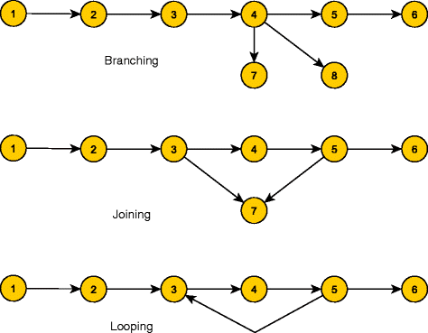
Branching, joining and looping operations. The operations that the parameterized graph generator do according to the parameters.
-
Joining: from two non-leaf different random nodes x and y, create a new node z and create two new edges (x,z) and (y,z));
-
Looping: from two non-leaf different random nodes x and y, with d e p t h(x)>d e p t h(y), create a new edge (x,y)).

The generator executes the same process as many times as the number of graphs to generate parameter indicates.
4.2.3 Data analysis
Since we divide the whole experiment into three similar experimental designs, the data analysis will respect this division and we follow the same chain of tests for the designs. Firstly, we test the normality assumptions over the samples using the Anderson-Darling and visual QQ-Plot tests and the equality of variances through Bartlett test. Depending on the result of these tests, we choose the next one, which evaluate the equality of the samples, Kruskal-Wallis or ANOVA. After evaluate the levels separately, we test the techniques isolatedly through the three levels. We consider for every test the significance level of 5%.
The objective in this work is to expose influences of the studied structural aspects of the models on the performance of the techniques, thus if the p-value analysis in a hypothesis testing suggests that the null hypothesis of equality may not be rejected, this is an evidence that the variable considered alone does not affect the performance of the techniques. On the other hand, if the null hypothesis must be rejected, it represents an evidence of some influence.
4.2.3.1 Branches analysis
The first activity for the analysis is the normality test and Table 6 summarizes this step. Among the samples, just the three with p-values in boldface have their null hypotheses of normality not rejected, which implies that a minor part of the samples was considered normal.
Following the analysis, we perform three tests, as summarized in the Table 7. We select the test according to the normality from the samples: for normal samples, we verify the variances of the samples, and perform the Analysis of Variance (ANOVA) and for non-normal samples, the Kruskal-Wallis test. All the p-values are greater than the defined significance of 5%, so the null hypothesis of equality of the techniques cannot be rejected, at the defined significance level, in other words, the four techniques presented similar performance at each level separately.
The next step of the analysis is to evaluate each technique separately through the levels and we proceed a non-parametric test of Kruskal-Wallis to test their correspondent hypothesis. The tests calculate for ART_Jac, ART_Man, Fixed_Weights and Stoop the p-values 0.2687, 0.848, 0.856 and 0.5289 respectively. Comparing them against the significance level of 5%, we cannot reject the null hypothesis of equality between the levels for each technique, so the performance is similar, at this significance level.
4.2.3.2 Joins analysis
Following the same approach from the first experimental design, we can see on Table 8 the p-values of the normality tests. The bold face p-values indicate the samples normally distributed, at the considered significance.
Based on these normality tests, we test the equality of the performance of the techniques at each level and, according to Table 9, the techniques perform statistically in a similar way at all levels.
The next step is to assess each technique separately. The samples for ART_Jac, ART_Man, Fixed_Weights were considered normal, according Table 8, but presented different variances, violating an ANOVA assumption. Therefore, we executed Kruskal-Wallis tests comparing the three samples for ART_Jac, ART_Man, Fixed_Weights and Stoop and the p-value obtained was 0.2235, 0.7611, 0.6441 and 0.3936, respectively. Comparing with the significance level considered of 5%, the null hypotheses of equality were not rejected, what means the techniques behave similarly through the levels.
4.2.3.3 Loops analysis
Following the same line of argumentation, the first step is to evaluate the normality of the measured data and Table 10 summarizes these tests.
According to the results of the normality tests, we test the equality of the techniques at each level of this experimental design. As we can see on Table 11, the null hypotheses for 1 Loop, 3 Loops and 9 loops cannot be rejected because they have p-value greater than 5%, thus the techniques present similar behavior for all levels of the factor.
Analyzing the four techniques separately through the levels, we performed the non-parametric Kruskal-Wallis test, because the variances were not similar according to a Bertlett-Test. The p-values of the Kruskal-Wallis tests are 0.883, 0.9255, 0.3834 and 0.05507 for ART_Jac, ART_Man, Fixed_Weights and Stoop, respectively. These p-values, compared with the significance level of 5%, indicate that the null hypotheses of the considered pairs cannot be rejected, in other words, the techniques perform statistically similar through the different levels of the number of looping operations.
4.2.4 Threats to validity
About the validity of the experiment, we can point some threats. To the internal validity, we define different designs to evaluate separately the factors, therefore, it is not possible analyze the interaction between the number of joins and branches, for example. We do it because some of the combinations between the three variables might be infeasible, e.g. a model with many joins and without any branch.
Moreover, we do not calculate the number of repetitions in order to achieve a defined precision, because the execution would be infeasible (conclusion validity). The executed configuration took several days because some test suites were huge. To deal with this limitation, we limit the generation to 31 graphs for each experimental design and 31 failure attributions for each graph, keeping the balancing principle (Wohlin et al. 2000) and samples with size greater than, or equal to, 31 are wide enough to test for normality with confidence (Jain 1991) (Montgomery and Runger 2003).
Furthermore, we generate synthetic application models to deal with the problem of lack of applications, but, at the same time, this reduces the capability of representing the reality, threatening the external validity. To deal with this, we used structural properties, e.g. depth and number of branches, from existent models.
4.3 Experiment 3: the failure profile
This section contains a report of an experiment that aims at “analyzing general prioritization techniques for the purpose of observing the failure profile influence over the studied techniques, with respect to their ability to reveal failures earlier, from the point of view of the tester and in the context of Model-Based Testing”.
Complementing the definition, we postulate the following research hypothesis: “The general test case prioritization techniques present different abilities to reveal failures, considering that the test cases that fail have different profiles”. We are considering profiles as structural characteristics of the test cases that reveal failures.
4.3.1 Planning
We perform the current experiment in the same environment of the previous ones and the application models used in this experiment are a subset of the used in the second study. Since we do not aim at observing variations of model structure, we consider the 31 models that we generated in the second experiment, with 30 branches, 15 joins, 1 loop and maximum depth 25.
For this experiment, we define these variables:
Independent variables
-
General prioritization techniques (factor): ART_Jac, ART_Man, Fixed_Weights, and Stoop;
-
Failure profiles, i.e., characteristics of the test cases that fail (factor);
-
Long test cases – with many steps (longTC);
-
Short test cases – with few steps (shortTC);
-
Test cases that contains many branches (manyBR);
-
Test cases that contains few branches (fewBR);
-
Test cases that contains many joins (manyJOIN);
-
Test cases that contains few joins (fewJOIN);
-
Essential test cases (ESSENTIAL) (the ones that uniquely covers a given edge in the model);
-
-
Number of test cases that fail: fixed value equals to 1;
Dependent variable
-
Average Percentage of Fault Detection - APFD.
A special step is the failure assignment, according to the profile. As the first step, the algorithm sorts the test cases according to the profile. For instance, for the longTC profile, the test cases are sorted decreasingly by the length or number of steps. If there are more than one with the biggest length (same profile), one of them is chosen randomly. For example, if the maximum size of the test cases is 15, the algorithm selects randomly one of the test cases with size equals to 15.
Considering the factors, this experiment is a one-factor-at-a-time, and we may proceed the analysis between the techniques at each failure profile and between the levels at each technique. In the execution of the experiment, each one of the 31 models were executed with 31 different and random failure assigned to each profile, with just one failure at once (a total of 961 executions for each technique). This number of repetitions keeps the design balanced and gives confidence for testing normality (Jain 1991).
Based on these variables and in the design, we define the correspondent pairs of statistical hypotheses: i) to analyze each profile with the null hypothesis of equality between the techniques and the alternative indicating they have a different performance (e.g. Considering \(T=\{ART\_Jac, ART\_Man, Fixed\_Weights, Stoop\}\phantom {\dot {i}\!}\), \(H_{0} :n{(t_{1},longTC)} = APFD_{(t_{2},longTC)}, \forall t_{1},t_{2} \in T\phantom {\dot {i}\!}\) and \(H_{1}: APFD_{(t_{1},longTC)} \neq APFD_{(t_{2},longTC)}, \exists t_{1}, t_{2} \in T\phantom {\dot {i}\!}\)), and also ii) to analyze each technique with the null hypothesis of equality between the profiles (e.g. Considering P={l o n g T C, s h o r t T C, m a n y B R, f e w B R, m a n y J O I N, f e w J O I N, E S S E N T I A L}, \(H_{0} : APFD_{(ARTJac,p_{1})} = APFD_{(ARTJac,p_{2})}, \forall p_{1},p_{2} \in P\phantom {\dot {i}\!}\) and \(H_{1} : APFD_{(ARTJac,p_{1})} \neq APFD_{(ARTJac,p_{2})}, \exists p_{1}, p_{2} \in P\phantom {\dot {i}\!}\)). Whether the tests reject null hypotheses, we will consider it as an evidence of the influence of the failure profile over the techniques.
The experiment execution follows the same steps defined to the model structure experiment. However, as mentioned before, each technique runs by considering one failure profile at a time.
4.3.2 Data analysis
By analyzing the profiles separately to test the first set of hypotheses, it is possible to visualize in the boxplots from Figures 5 and 6, significant differences among the techniques, represented by some lack of overlap among the notches in the boxplots. The notches in the boxplots are a graphical representation of a confidence interval calculated by the R software. When these notches overlap, it suggests a better and deeper investigation of the statistical similarity of the samples. Thereby, the boxplots in the figures already mentioned are enough to reject every null hypotheses of the first set, in another words, the techniques perform different at each failure profile isolatedly.

Boxplots with the samples from Long_TC, Short_TC, Many_BR and Few_BR. The boxplots of the samples of the techniques associated with the Long_TC, Short_TC, Many_BR and Few_BR profiles.

Boxplots with the samples from Many_JOIN, Few_JOIN and ESSENTIAL. The boxplots of the samples of the techniques associated with the Many_JOIN, Few_JOIN, and ESSENTIAL profiles.
For testing the second set of hypotheses, from a visual analysis of the boxplots of the samples in Figure 7, we can see that there are profiles that do not overlap for each technique, thus the null hypotheses of equality must be rejected. In other words, at 5% of significance, ART_Jac, ART_Man, Fixed_Weights and Stoop perform statistically different for every researched profile.

Boxplots with the samples from the techniques. Boxplot summarizing the data collected from the executions of all techniques.
As a secondary analysis, by observing the profiles longTC and manyBR, in Figure 5, they incur in similar performances for the techniques, because frequently a test case among the longest ones are also among the ones with the biggest number of branches. The same happens with the profiles ShortTC and FewBR, by the same reason.
In summary, the rejection of every null hypothesis of equality is a strong evidence of the influence of the failure profiles over the performance of the general prioritization techniques. Furthermore, data suggests that the techniques may present better and worse performances with different failure profiles.
4.3.3 Threats to validity
Regarding conclusion validity, we do not calculate the number of repetitions needed to achieve a defined precision, we limited the random failure attributions at each profile for each graph in 31, keeping the balancing principle (Wohlin et al. 2000) and samples with size greater than, or equal to, 31 are wide enough to test for normality with confidence (Jain 1991) (Montgomery and Runger 2003).
Construct validity is threatened by the definition of the failure profiles. We choose the profiles based on data and observations from previous studies, not necessarily the specific results. Thus, we define them according to our experience and there might be other profiles not investigated yet. This threat is reduced by the experiment’s objective, which is just to expose the influence of different profiles on the prioritization techniques performance, and not to show all possible profiles.
5 Results and Discussion
Analyzing the first study (refer to Section 1), even though we cannot expect to know precisely the rate of failure of a system before test execution, it is worthy investigating how techniques perform when more or less failures occur. It is often possible to predict failure rate by analyzing the application history or even similar applications. Based on prediction, a tester can choose the technique that presents the best behavior.
By varying the number of test cases that fail, we can observe differences on the performance of the techniques. However, we may not be confident to use only this information when choosing a technique. On one hand, from the results of the motivational study, techniques based on random choice have a best performance when the rate of failure is low, whereas Stoop increases performance as the rate of failures increase and Fixed_Weights increases performance when the level goes from medium to high. On the other hand, growth rates do not follow a pattern as well as they are not regular. Furthermore, Stoop and Fixed Weights are mostly based on structural elements of the test cases and their performance present different patterns. Thus, these results are consonant with our research hypothesis, which stated that prioritization techniques present different abilities of revealing failures, varying the amount test cases that fail in the test suite, motivating the investigation of the influence of the structure of the model.
For the first experiment, considering models with different structures such as branches, joins and loops (refer to Section 1), we expect that algorithms generate test cases with different lengths. For instance, cascade branches (or branches distributed at different levels of the model structure) may lead to a variety of short to long test cases. Moreover, we expect that test cases may be more or less redundant with respect to covering common transitions, particularly the more branches, joins and loops the model has, more redundancy the test cases have since they might cover common prefix of the branches and joins as well as repetitive sequences of loops. Since the techniques investigated either focus on the use of distance functions or on the presence of certain structures explicitly, we expect that by focusing on certain structure patterns, we could observe related behavior from the techniques.
Nevertheless, the configurations of structures we considered for each treatment of the independent variables do not show statistical difference on the behavior of the studied techniques, leading us to reject our initial research hypothesis, which stated that the prioritization techniques present different performances considering models with specific structures.
It is important to remark that each configuration considered may represent specific kinds of applications. For example, at system level: i) more branches may indicate the prevalence of alternate and exception flows that do not join with the main flow of the application; ii) more joins may indicate the prevalence of alternate and exception flows that join with the main flow; and iii) more loops may indicate the prevalence of repetitive cycles of execution. In practice, the distribution of these structural elements in the model depends on the system behavior as well as on the level of modeling. Overall, results show that from a practical point of view, only based on the structure of the model, we are unable to define what is the most effective technique to execute.
By closely analyzing the model for each configuration, we realize that results are influenced only if the test cases that fail cover the structure. This observation motivates the execution of the experiment presented in Section 1.
However, in the second experiment (refer to Section 1), we already had some intuition about techniques being more successful in determined situations, through less controlled studies, but now we have evidence supporting it. These techniques are sensitive to test cases that fail with different characteristics, as proposed by the data analysis, since techniques may perform well with failures with a characteristic and bad with another scenario.
As an example of how the profile of the test case that fail may influence on the performance of the technique, consider one of the models from our study as presented in Figure 8. From this model, consider a short test case T 1=(A W).

Example model among the objects of the experiment. A model that composes the sample used in the third experiment reported in this paper.
For this test case, for example, the APFD values obtained in the first trial by the ART_Jac and Stoop techniques are 0.8373 and 0.0060 respectively. This is because ART_Jac selects, among the candidates, the test case with the highest minimum distance to the already prioritized ones and, as soon as T 1 appear in the candidate set, it is chosen. On the other hand, the Stoop technique focus on test cases with more common steps and, since T 1 has just one step and it is unique, this test case is placed in the end of the sequence.
Now, consider the following long test case: T 2=(A,B,C,D,E,F,G,H,I,J,K,L,M,N,O,P,Q,R,S,T,U,V,W,X,Y). For this test case, the APFD values obtained in the eighth trial for ART_Jac and Stoop techniques are 0.0662 and 0.1144 respectively. This is because ART_Jac takes into account the number of branches in common in order to select the next test case, through the Jaccard function, and, since T 2 has more chance to have more branches in common with other already prioritized test case, it will appear just in the end of the sequence. On the other hand, the Stoop technique quickly returns it since it has many common steps with the other test cases.
After this study, the factor “failure profile” must be considered into any further evaluation of prioritization techniques, since it is an important factor for explaining the performance of prioritization techniques. Its importance corroborates our initial research hypothesis, which stated that prioritization techniques present different abilities of reveal failures, varying the characteristics of the test cases that fail.
6 Conclusions
This paper presents and discusses the results obtained from empirical studies about test case prioritization techniques in the context of MBT. Furthermore, this paper is an extension of the study presented in (Ouriques et al. 2013) and gives more evidences favoring the proposed results, since the conclusions are the same. It is widely accepted that a number of factors may influence on the performance of the techniques, particularly because the techniques can be based on different aspects and strategies, including or not random choice.
In this sense, the main contribution of this paper is to investigate the influence of two factors: the structure of the model and the profile of the test case that fails. The intuition behind this choice is that the structure of the model may determine the size of the generated test suites and the redundancy degree among their test cases.
Therefore, this factor may affect all of the techniques involved in the experiment due to either the use of distance functions or the fact that the techniques consider certain structures explicitly. On the other hand, depending on the selection strategy, the techniques may favor the selection of given profiles of test cases despite others. Thereby, whether the test cases that fail have a certain structural property may also determine the success of a technique. To the best of our knowledge, there are no similar studies presented in the literature.
In summary, in the first study, since we perform the experiment with real applications in a specific context, different growth patterns of APFD for the techniques compose an evidence of influence of more factors in the performance of the general prioritization techniques other than the number of test cases that fail. This result motivated the execution of the other studies.
On one hand, the second study, which aims at investigating the influence of the number of occurrences of branches, joins, and loops over the performance of the techniques, shows that there is no statistical difference on these performances, considering a significance of 5%. On the other hand, in the third study, based on the profile of the test case that fail, the fact that all of the null hypotheses must be rejected may indicate a high influence of the failure profile on the performance of the general prioritization techniques.
Moreover, from the perspective of the techniques, this study exposed weaknesses associated with the profiles. For instance, ART_Jac presented low performance when long test cases (and/or with many branches) reveal failures and high when short test cases (and/or with few branches) reveal failures. On the other hand, Stoop showed low performance with almost all profiles.
Overall, the results may contribute the improvement of prioritization techniques by addressing the weaknesses exposed. However, from a practitioner point of view, we do not have enough data to provide guidelines to apply the techniques yet. Generally, the results obtained point to a tendency that knowledge of which technique performs better for a given profile can be worthy if the team have some assumption about the characteristics of the test cases that fail. For example: if they have the assumption that test cases that cover more branches are more likely to fail because they go through many conditions, then it can be better to use Fixed Weights.
As future work, we will perform a more complex factorial experiment, calculating the interaction between the factors analyzed separately in the experiments reported in this paper. Moreover, we plan an extension of the third experiment to consider other profiles of test cases that may be of interest. From the analysis of the results obtained, a new (possibly hybrid) technique may emerge.
7 Endnotes
a A number of loops distributed in a model may lead to huge test suites with a certain degree of redundancy between the test cases even if they are traversed only once for each test case.
b The pseudomedian is a non-parametric estimator for the median of a population (Lehmann 1975).
References
Aho, AV, Hopcroft JE, Ullman JD (1974) The Design and Analysis of Computer Algorithms. Addison-Wesley, Massachusetts, USA.
Cartaxo, EG, Andrade WL, Neto FGO, Machado PDL (2008) LTS-BT: a tool to generate and select functional test cases for embedded systems In: SAC ’08: Proc. of the 2008 ACM Symposium on Applied Computing,1540–1544.. ACM, New York, NY, USA.
Cartaxo, EG, Machado PDL, Neto FGO (2008) Seleção automática de casos de teste baseada em funções de similaridade In: XXIII Simpósio Brasileiro de Engenharia de Software,1–16.
Cartaxo, EG, Machado PDL, Oliveira FG (2011) On the use of a similarity function for test case selection in the context of model-based testing. Software Test Verification Reliability 21(2): 75–100.
Chen, TY, Leung H, Mak IK (2004) Adaptive random testing In: Advances in Computer Science - ASIAN 2004. Lecture Notes in Computer Science,320–329.. Springer, Auckland, New Zealand.
Cormen, TH, Leiserson CE, Rivest RL, Stein C (2009) Introduction of Algorithms, 3rd edn. MIT Press, Massachusetts, USA.
de Lima, LA (2009) Test case prioritization based on data reuse for black-box environments. Master’s thesis, Universidade Federal de Pernambuco.
de Vries, RG, Tretmans J (2000) On-the-fly conformance testing using spin. International Journal on Software Tools for Technology Transfer 2(4): 382–393.
Do, H, Mirarab S, Tahvildari L, Rothermel G (2010) The effects of time constraints on test case prioritization: A series of controlled experiments. IEEE Trans Software Eng 36(5): 593–617.
Elbaum, S, Malishevsky AG, Rothermel G (2000) Prioritizing test cases for regression testing In: Proceedings of the 2000 ACM SIGSOFT International Symposium on Software Testing and Analysis. ISSTA ’00,102–112.. ACM, New York, NY, USA,
Elbaum, SG, Malishevsky AG, Rothermel G (2002) Test case prioritization: A family of empirical studies. IEEE Transactions in Software Engineering 26(2): 159–182.
Elbaum Sebastian, Rothermel Gregg, Kaduri Satya, Malishevsky Alexey G (2004) Selecting a cost-effective test case prioritization technique. Software Qual J 12: 2004.
Gopinathan Sapna, Ponaraseri, Mohanty H (2009) Prioritization of scenarios based on uml activity diagrams In: CICSyN,271–276.
Gomes de, OliveiraNeto, F, Feldt R, Torkar R, Machado PDL (2013) Searching for models to evaluate software technology In: Combining Modelling and Search-Based Software Engineering (CMSBSE), 2013 1st International Workshop On, 12–15.. IEEE, San Francisco,
Harrold, MJ, Gupta R, Soffa ML (1993) A methodology for controlling the size of a test suite. ACM Trans Softw Eng Methodol 2(3): 270–285.
Ouriques, JFS, Cartaxo EG, Machado PDL (2015) Empirical Studies on Model-Based Testing Prioritization. https://sites.google.com/a/computacao.ufcg.edu.br/mb-tcp/. Acessed in 21 Jan 2015.
Gentleman, R, Ihaka R (2015) The R Project for Statistical Computing. http://www.r-project.org/. Acessed in 21 Jan 2015.
Vacondio, A, Bortolotti E, Benblidia H (2015) PDF Split and Merge. http://www.pdfsam.org. Acessed in 21 Jan 2015.
National Institute of Software Engineering (2015). www.ines.org.br. Acessed in 21 Jan 2015.
Jain, RK (1991) The Art of Computer Systems Performance Analysis: Techniques for Experimental Design, Measurement, Simulation, and Modeling. Wiley, New York, NY, USA.
Jeffrey, D (2006) Test case prioritization using relevant slices In: In the Intl. Computer Software and Applications Conf, 411–418.. IEEE, Chicago,
Jeffrey, D, Gupta R (2007) Improving fault detection capability by selectively retaining test cases during test suite reduction. Software Eng IEEE Trans 33(2): 108–123.
Jiang, B, Zhang Z, Chan WK, Tse TH (2009) Adaptive random test case prioritization In: Automated Software Engineering, 233–244.. IEEE, Auckland,
Korel, B, Koutsogiannakis G, Tahat LH (2007) Model-based test prioritization heuristic methods and their evaluation In: Proceedings of the 3rd International Workshop on Advances in Model-based Testing A-MOST ’07, 34–43.. ACM, New York, NY, USA,
Korel, B, Koutsogiannakis G, Tahat LH (2008) Application of system models in regression test suite prioritization In: IEEE International Conference on Software Maintenance, 247–256.. IEEE, Beijing,
Korel, B, Tahat LH, Harman M (2005) Test prioritization using system models In: Software Maintenance, 2005. ICSM’05. Proceedings of the 21st IEEE International Conference On, 559–568.. IEEE, Budapest,
Kundu, D, Sarma M, Samanta D, Mall R (2009) System testing for object-oriented systems with test case prioritization. Softw Test Verif Reliab 19(4): 297–333.
Lehmann, E (1975) Nonparametrics: Statistical Methods Based on Ranks. Holden-Day series in probability and statistics. Holden-Day, San Francisco.
Montgomery, DC, Runger GC (2003) Applied Statistics and Probability for Engineers. John Wiley and Sons, New York, NY, USA.
Ouriques, JFS (January 2012) Análise comparativa entre técnicas de priorização geral de casos de teste no contexto do teste baseado em especificação. Master’s thesis, UFCG.
Ouriques, JFS, Cartaxo E, Machado PDL (2010) Comparando técnicas de priorização de casos de teste no contexto de teste baseado em modelos In: Proceedings of the IV Brazilian Workshop on Systematic and Automatic Software Testing (SAST 2010).. UFRN, Natal.
Ouriques, JFS, Cartaxo EG, Machado PDL (2013) On the influence of model structure and test case profile on the prioritization of test cases in the context of model-based testing In: Proceedings of XXVII Brazilian Symposium on Software Engineering,134–143.. UnB, Brasilia,
Rothermel, G, Untch RH, Chu C, Harrold MJ (1999) Test case prioritization: an empirical study In: Software Maintenance, 1999. (ICSM ’99) Proceedings. IEEE International Conference On, 179–188.. IEEE, Oxford,
Rothermel, G, Untch RH, Chu C, Harrold MJ (2001) Prioritizing test cases for regression testing. IEEE Trans Software Eng 27: 929–948.
Utting, M, Legeard B (2007) Practical Model-Based Testing - A Tools Approach. Morgan Kaufmann, San Francisco, CA, USA.
Wohlin, C, Runeson P, Host M, Ohlsson MC, Regnell B, Wesslen A (2000) Experimentation in Software Engineering: an Introduction. Kluwer Academic Publishers, Norwell, MA, USA.
Wu, CFJ, Hamada MS (2009) Experiments: Planning, Analysis, and Optimization. 2nd edn. John Wiley and Sons, New York, NY, USA.
Yoo, S, Harman M, Tonella P, Susi A (2009) Clustering test cases to achieve effective and scalable prioritisation incorporating expert knowledge In: Proceedings of the Eighteenth International Symposium on Software Testing and Analysis. ISSTA ’09,201–212, New York, NY, USA,
Zhou, ZQ (2010) Using coverage information to guide test case selection in adaptive random testing In: IEEE 34th Annual COMPSACW, 208–213.. IEEE, Seoul.
Zhou, ZQ, Sinaga A, Susilo W (2012) On the fault-detection capabilities of adaptive random test case prioritization: Case studies with large test suites In: HICSS,5584–5593.. IEEE, Maui,
Acknowledgements
This work was supported by CNPq grants 484643/2011-8 and 560014/2010-4. Also, this work was partially supported by the National Institute of Science and Technology for Software Engineering (2015), funded by CNPq/Brasil, grant 573964/2008-4. First author was also supported by CNPq.
Author information
Authors and Affiliations
Corresponding author
Additional information
Competing interests
The authors declare that they have no competing interests.
Authors’ contributions
JF idealized the studies, implemented the techniques and the scripts for data analysis. EG helped in the project of the experiments and reviewed the paper. PD reviewed the initial draft and the final version of the paper. All authors read and approved the final manuscript.
Rights and permissions
Open Access This article is licensed under a Creative Commons Attribution 4.0 International License, which permits use, sharing, adaptation, distribution and reproduction in any medium or format, as long as you give appropriate credit to the original author(s) and the source, provide a link to the Creative Commons licence, and indicate if changes were made.
The images or other third party material in this article are included in the article’s Creative Commons licence, unless indicated otherwise in a credit line to the material. If material is not included in the article’s Creative Commons licence and your intended use is not permitted by statutory regulation or exceeds the permitted use, you will need to obtain permission directly from the copyright holder.
To view a copy of this licence, visit https://creativecommons.org/licenses/by/4.0/.
About this article

Cite this article
Silva Ouriques, J.F., Cartaxo, E.G. & Lima Machado, P.D. Revealing influence of model structure and test case profile on the prioritization of test cases in the context of model-based testing. J Softw Eng Res Dev 3, 1 (2015). https://doi.org/10.1186/s40411-014-0015-5
Received:
Accepted:
Published:
DOI: https://doi.org/10.1186/s40411-014-0015-5